TensorFlow is an open-source software library for machine learning developed by researchers and engineers working on the Google Brain Team. The first publicly available version was released in Novembre 2015. TensorFlow quickly became popular in the deep learning community for several reasons. The main reason might be that TensorFlow is maintained by a professional developer team (whereas Caffe, Theano, … are developed by academic researchers). I won’t discuss the pros and the cons of the different machine learning frameworks here. It is not the point! A good rule of thumb is to check how many stars/fork TensorFlow got on Github. According to the number of Stars/Forks of GitHub we can guess that TensorFlow has the biggest community!

Installing Tensor on Windows

When Google decided to release its library under the Apache 2.0 open source license, TensorFlow was primarily available on Mac and Linux. After several months, TensorFlow was finally available on Windows. However, it is much easier to use TensorFlow on Linux Operating System then on Windows. That is why I will only focus on how to install TensorFlow on Windows Operating System. Firstly, We should notice that, at the time I’m writing this article, TensorFlow is only available for Python 3.5 on Windows (while on Linux and Mac You can use TensorFlow with Python 2.7 for example).

Installing the CPU version

To install TensorFlow on Windows the easiest way is to install Anaconda. The steps are:

1. Download Anaconda for Windows. Install Python 3.X version (at the time I’m writing the tutorial the version is Python 3.6)
2. Launch the installer and install Anaconda
3. Once the installation is finished go to Windows and type Anaconda. Finally, click on Anaconda Prompt.
   

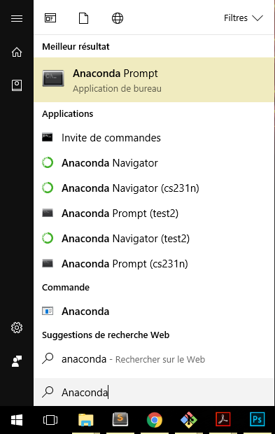   Anaconda Prompt under Windows 10
4. Once the Prompt is open we will need to create an environment for Python 3.5 (because TensorFlow is not available on Python 3.6 yet). To create an environment, simply type:

   conda create --name tensorflow python=3.5 anaconda
   

   This command will create a Python 3.5 environment named tensorflow.

5. We then activate the environment we’ve just created using:

   activate tensorflow
   

   On Linux, Mac, and Git for Windows we need to write source activate tensorflow.

6. We then install common package like jupyter and scipy (scipy will install numpy) and tensorflow using:

   conda install jupyter
   conda install scipy
   pip install tensorflow
   

So now we can use TensorFlow on Windows. Yet if you have a good Nvidia GPU, you might want to use it with TensorFlow. Indeed TensorFlow supports CUDA Drivers and using TensorFlow on GPU might increase the speed of your training phase by 10 or more.

Installing the GPU version

To install the GPU version of Windows you will firstly need to install:

• CUDA Drivers
• cuDNN

The steps are:

1. Download CUDA for your operating system
2. Launch the installer and install CUDA
3. Then download cuDNN¹. You might need to create an nvidia account before downloading cuDNN.
4. Unzip the archive. You should get a folder containing 3 other folders:
   • bin
   • include
   • lib
5. Go to C:\ and create a folder named Cuda, then copy and paste the folders bin, include, lib inside your Cuda folder. You should have something like this: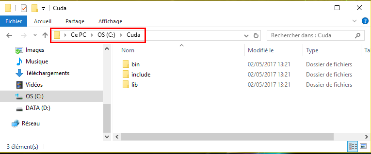
   

   folders bin, include, lib are under C:\Cuda
6. Now add C:\Cuda to your Path environment variable. To do so:
   • Right Clikc on Windows -> System -> Advanced system settings (on the left) -> Environment Variables
   • Click on Path Variable under System Variables and then click Edit... and Add ;C:\Cuda at the end of the Path variable. (On windows 10 you will just have to add C:\Cuda on a new line). here is a screenshot:
   

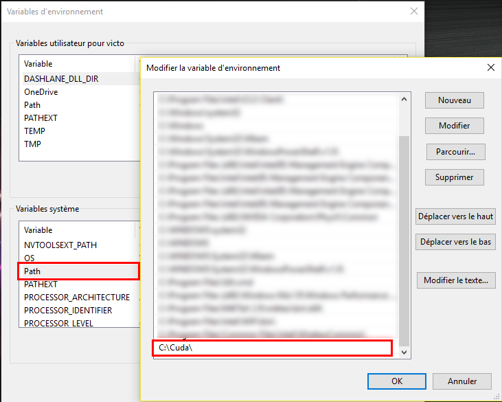   Adding C:\Cuda to Path variable
7. Launch Anaconda Prompt: Windows -> type Anaconda -> Click on Anaconda Prompt
8. create a GPU TensorFlow environment, using:

   conda create --name tensorflow-gpu python=3.5 anaconda
   

9. activate the environment named tensorflow-gpu

   activate tensorflow-gpu
   

10. Install jupyter and scipy and other package if you want
11. Install tensorflow for GPU using:

    pip install --ignore-installed --upgrade https://storage.googleapis.com/tensorflow/windows/gpu/tensorflow_gpu-1.1.0-cp35-cp35m-win_amd64.whl
    

Note: if you tried to install TensorFlow using pip install tensorflow-gpu you might encounter an error. To solve this issue you need to download Microsoft Visual C++ 2015 Redistributable

Should I use my CPU or my GPU?

Now that we sucessfully installed both the CPU and GPU versions of TensorFlow, we might wonder which version you should use. The easy answer is: use the GPU version

To understand why you should use your GPU over your CPU, you should first understand what is the difference between a GPU and a CPU.

• CPU stands for Central Processing Unit and CPUs are optimized for Serial Tasks. We will prefer to use CPUs over GPUs for any sequence of task that are not easily parallelisable. For example we will prefer to use a CPU when we are dealing with non trivial recusive tasks. Hence, we will prefer to use CPUs for RNN because RNN are made of Recursive Task: We cannot compute the next term before having computed the previous term (see figure below).

Figure 1: Architecture of a RNN. We can see that to compute $h_{n+1}$
we need to have computed $h_{n}$. Hence this task is somehow recursive

• GPU stands for Graphics Processing Unit and GPUs are optimized for Parallel Tasks. We will prefer to use GPUs over CPUs when we can divide the main task into several tasks that we can compute in parallel. We will therefore prefer to use GPUs for CNN because CNN are made of several subtasks that we can compute independaly from each others (see figure below).

The source image is split into 3 images. One for each RGB layer. Then we convolve each Red, Blue, Green layer< with a filter and we obtain 3 activation maps (red, blue, green parallelepipeds in the image). One for the blue layer, one for the red layer and one for the green layer. The convolution of each layer can be made in parallel. Moreover the convolution of each part of the image with a filter can also be made in parallel.

So, according to what I’ve just said you might think that it is better to use a CPU for RNN and a GPU for CNN. Well, actually it is not that simple. Indeed we can parallelize tasks in a RNN with a certain trade-off. I won’t enter into any detail but there are many ways (other than just by increasing parallelism) we can improve the performance of RNN on GPUs. We can for example:

• Reduce the memory traffic
• Reduce overheads
• Increase the parallelism

So in general, whether you are dealing with CNN or RNN or any other types of Neural Network, it will be preferable to use your GPU (supposing you have a good Nvidia GPU of course!)

Introducing TensorFlow Concepts

To better understand how TensorFlow works, we can represent any operation as a Flow Graph where each node of the graph represents mathematical operations and each edge represents the tensor communicated between them. You can think of a Tensor as a list, an array or a multidimensional array.

Example of a simple Flow Graph that we can compute using TensorFlow. The Red circle represents the data we feed to the Neural Network (Placeholder in TensorFlow). The Blue circles represent the parameters we want to update during training (Variables in TensorFlow). The gray circles represent the mathematical operations we can perform between tensors. The edges represent the tensors flowing through the graph.

Variables, Placeholders, Mathematical Operations

• Variables are stateful nodes. Each time we need to create a parameter (Weight matrix, bias term, …) we will create a Variable in TensorFlow. For example, we can create a matrix of weights $ W \in \mathbb{R}^{784 \times 100}$ and a bias term $b \in \mathbb{R}^{100}$ with:

import tensorflow as tf

W = tf.Variable( tf.random_uniform((784, 100), -1, 1) )
b = tf.Variable( tf.zeros((100,)) )

• Placeholders are nodes whose value is fed in at execution time. Hence we will create a placeholder for any data that our model take as inputs or ouputs: inputs, labels,… For example, assuming we have a input vector of length 784 and that we are working with a mini-batch of size 100, we will create our input $x \in \mathbb{R}^{100 \times 784}$ using:

x = tf.placeholder(tf.float32, (100, 784))

• Mathematical Operations. Any Mathematical operations are implemented using built-in functions from TensorFlow. For example to multiply two matrices we can use matmul(). If we want to use a ReLu activation function we can use the relu() function. Hence to compute $h = ReLu(Wx + b)$ we can write:

h = tf.nn.relu( tf.matmul(x, W) + b )

Here is the final code snippet:

import tensorflow as tf

W = tf.Variable( tf.random_uniform((784, 100), -1, 1) )
b = tf.Variable( tf.zeros((100,)) )

x = tf.placeholder(tf.float32, (100, 784))

h = tf.nn.relu( tf.matmul(x, W) + b )

Fetch, Feed

Now that we’ve built our skeleton, we will now need to run a session to get our outputs. A session is a binding to a particular execution context (CPU, GPU, …). To initialize a session we can simply use:

session = tf.Session()

To initialize the Variables, we can then use the built-in function tf.initialize_all_variables():

session.run(tf.initialize_all_variables())

So now we have initialized our session and our variables (Weight matrix and bias here), but we still didn’t initialize our data (inputs, labels, …). We created a placeholder that can accept a data of shape $(100, 784)$ but we still didn’t feed this data and we still didn’t specify which outputs we want to retrieve. To do so we will use the session.run(fetches, feeds) function where:

• Fetches is a list of graph nodes that we want to retrieve.
• Feeds is a dictionary mapping from graph nodes to concrete values. Hence Feeds can be seen as a dictionary mapping each placeholder to their values.

As we want to retrieve our output h and as we only have one placeholder x we can finally run our session using:

session.run(h, {x: np.random.random(100, 784)})

and the full code snippet is:

import tensorflow as tf

W = tf.Variable( tf.random_uniform((784, 100), -1, 1) )
b = tf.Variable( tf.zeros((100,)) )

x = tf.placeholder(tf.float32, (100, 784))

h = tf.nn.relu( tf.matmul(x, W) + b )

session = tf.Session()
session.run(tf.initialize_all_variables())
session.run(h, {x: np.random.random(100, 784)})

Adding the loss

In order for the model to compute the loss and update the weight matrix and bias term accordingly, we will just need to specify a loss function and which optimizer we want to use. I will keep things simple and only use the basic cross_entropy loss function and the simple stochastic gradient descent. To train our model we then define our cross_entropy loss using:

cross_entropy = -tf.reduce_sum(label * tf.log(prediction), axis=1)

we then create an optimizer using tf.train.GradientDescentOptimizer(learning_rate) and we pass our loss (here cross_entropy) to the minimize method of our optimizer. In python we have finally:

optimizer = tf.train.GradientDescentOptimizer(0.1) # 0.1 is the learning rate
train_step = optimize.minimize(cross_entropy)

Training the Model

Finally to train the model we can simply iterate over each batch of our data and pass train_step as our fetch and initialize our feed dictionary. In Python, assuming we have created a function that gives use the next batch of data we can write:

for i in range(200):
	batch_x, batch_label = data.next_batch()
	session.run(train_step, feed_dict={x: batch_x, label: batch_label} )