In the previous article we have seen the MCTS algorithm. this algorithm and all its variations have been used to create a lot of AI for the game of Go. Indeed, AlphaGo Zero, the first Artificial Intelligence that was able to learn without the need of human supervision still use a variant of this algorithm. In this article, I will explain how a Convolutional Neural Networks work. This is a necessary step if you want to understand how the AlphaGo Zero AI works! Are you ready? Follow me!

I. Filter

Before we deal with what we mean by filter, we need to explain how, in computer science, an image is formed. It depends of the color space in which we are working, but, usually, an image is made of 3 layers: the red, the green and the blue layers. In other words an image of size $600 \times 800$ is actually a tensor of size (600, 800, 3).

Each pixel is encoded with 3 values (red, blue, green). Each red, blue, green values are integer values in the range $[0, 255]$. For example:

• the red color is encoded by: (red$=255$, blue$=0$, green$=0$)
• the yellow color is encoded by (red$=255$, blue$=255$, green$=0$) because the yellow is a mix between the red and the blue color
• a metallic color can be encoded by (red$=188$, blue$=128$, green$=67$)

a pixel is usually just a mix of 3 colors (Red, Blue, Green). You just need to tell how much of each color you want. As each Red, Blue, Green values are in the range $[0, 255]$, it means that the number of possible colors you can display on a normal screen is actually $256 \times 256 \times 256 = 16777216$.

Figure I.1 shows a tensor representing an image of size $6 \times 10$

Figure I.1: An image can be represented as a tensor of $3$ dimensions. The first dimension is the height of the image, the second dimension corresponds to the width of the image and the last dimension correspond to the number of layers needed to encode a pixel. In general a pixel is coded with 3 colors (Red, Green, Blue) but it depends of the color space in which we are working.

The question is now:

A filter is just another tensor of arbitrary width and height and depth. It is a tensor, but it is not necessarily an image as this tensor might not always be interpreted as an image.

I know… this definition is quite vague, so let’s again explain it in more details. The width, height and depth of a filter are arbitrary which means that you choose the size of the filter! For example, let’s suppose I want a filter of size $3 \times 3 \times 1$. The question is:

This part is, again, completely arbitrary. Which means that you choose what to put in each cell of your filter. Of course we are in computer science, so you cannot put a cauliflower and a carrot in these cells. We will put numbers (be it integer or floating point), but you’ll be the one to choose which number to put in each cell!

Before moving on to the next subject where we will explain what a convolution is and how a filter can be used, let’s first define 2 common $3 \times 3$ filters:

Figure I.2: 2 common $3 \times 3$ filters

Yes, I know! A filter can still be very abstract to you, but don’t worry, once we will explain what is a convolution, you will understand how a filter can be used and hopefully understand how powerful they are.

II. Convolutions

Don’t worry a convolution is nothing too fancy. As always, as an image is worth 1000 words, let’s explain to you what a convolution is with a Figure. In our case we will say that a convolution is an operation between 2 tensors. In our example, the first tensor is the input image and the other is our filter. The convolution operation is explained on Figure II.1

Figure II.1: Convolution explained for one pixel

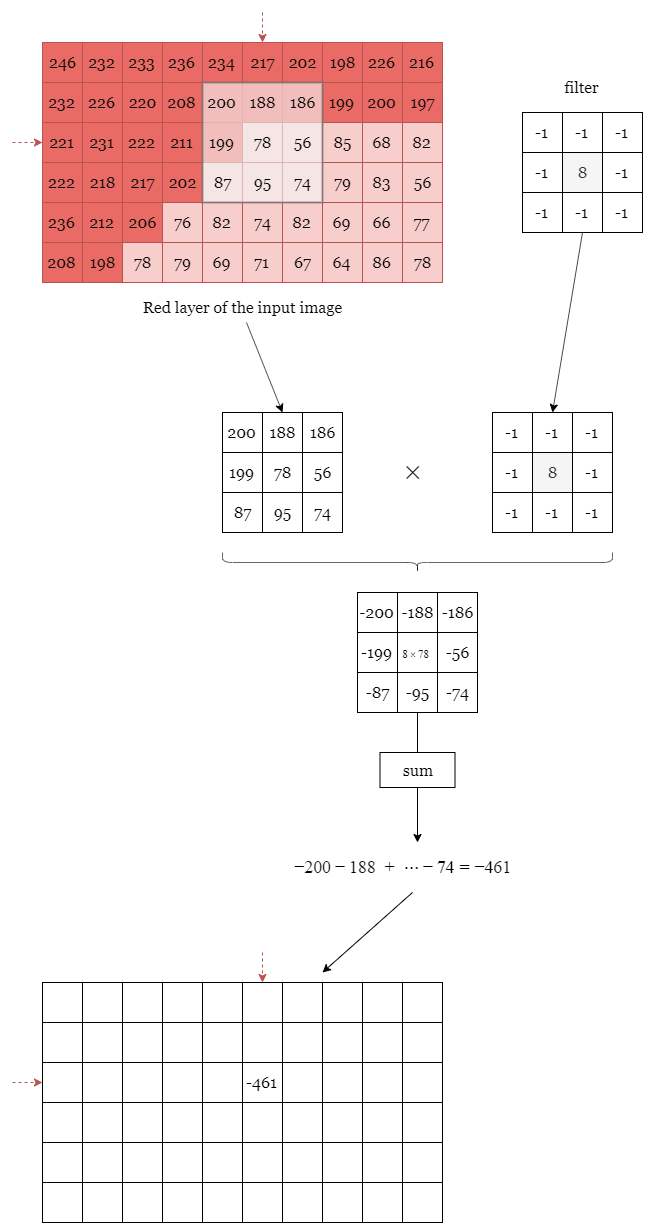
The idea is that we overlap the filter with a part of the input image. We then multiply all the pixel values with the coefficients of the filter. We finally sum all the values we got, and, in this example it gives us $-461$. We then put this number back in a tensor of the same size as the input image centered on the overlapping zone.

We need to do that with all the pixels. To handle the pixels on the border of the image, we can use different strategies. Use a mirror padding, use a $0$ padding, and so on. This is represented in Figure II.2.

Figure II.2: Pad the image before convolving it with the filter

Finally, if we use the symmetric padding strategy and if we overlap the filter with all the pixels of the input image, we will (you can do the calculation yourself) retrieve the following result:

Figure II.3: The result of convolving the red layer (with symmetric padding) and the filter. the blue cells are the cells that contain the biggest absolute value (greater than 250 or lower than -250 in our example).

Why did I highlight the cell with the biggest absolute values? Well, it’s simple. In the input image there are 2 kinds of red pixels. Pixels with a lot of red (a high value) and pixel with not a lot of red in it (pixel with a low value). You can see that after convolving the filter with the input image, the cells that I have highlighted in blue correspond roughly to the edges in the original image.

Let’s see a real case example to confirm our intuition that convolving this filter with an image, create a new image on which the edges are highlighted! Here is what we need to do:

• open an image
• transform the image into a grayscale image (we will only have a tensor of size (H, W) where H is the height of the image and W is the width of the image)
• convolve the filter with the input image
• take the absolute value of each value
• normalize the result and display the new image

For example, a very quick and dirty way do to it in python would be:

import numpy as np
import cv2
import matplotlib.pyplot as plt
import scipy.misc

from scipy.signal import convolve2d


input_image = cv2.imread("border_collie.jpg")
gray_image = cv2.cvtColor(input_image, cv2.COLOR_BGR2GRAY) / 255

fi = np.array([
    [-1, -1, -1],
    [-1, 8, -1],
    [-1, -1, -1]
])

conv = convolve2d(gray_image, fi, mode='same', boundary='symm')
abs_conv = np.absolute(conv)
clipped_result = np.clip(abs_conv, 0, 1.0)

plt.figure(figsize=(15, 20))
plt.imshow(clipped_result, cmap='gray')

scipy.misc.imsave("result_3x3.jpg", clipped_result)

If we apply such algorithm on an input image, here is what we get:

Figure II.4: convolve a $3 \times 3$ filter with the dog image

As we can see, our intuition is rather confirmed. We can see for example that the borders of the arm are well delimited, We can see also that the dog is well delimitated with respect to the green background. Moreover the white and black colors on the dog’s head are also quite apparent in the output. nevertheless the ears of the dog are not quite well distinguished from the background… So our intuition is wrong?

Well, this can easily be explained actually. The upper part of the image contains a focal blur which means that adjacent pixels to the center pixel have values that are not so dissimilar and hence our convolution fails to distinguish these edges.

Indeed, If all the pixels surrounding a central pixel have quite similar values, then, if we convolve it with the 2 filters we’ve introduced, we will get a number close to $0$. Moreover we have seen that an edge corresponds to a high absolute value. $0$ is certainly not a high absolute value!

One quick idea to fix this issue is to use a bigger filter that accounts for more than just the immediate adjacent pixels. Indeed, with a focal blur, adjacent pixels have values that are quite similar but pixels that are $2$ pixels away should have more dissimilar values (it depends on the strength of the blur of course).

If we use a bigger filter, here is what we obtain:

Figure II.5: convolve a $5 \times 5$ filter with the dog image

As you can see, we have a better result. We can see the nose of the dog, the ears, the teeth and yet the background remains black, the interior of the arm remain mostly black too as these regions are formed with quite similar pixels.

Filters and convolutions are inseparable in image processing. Maybe, it is possible to find a filter that will be able to separate the nose of the dog from everything else? It would be incredible, isn’t it? The problem is that, as I told you. The filters are arbitrary, which means that we need to find these filters ourself! Building a filter to highlight the edges in an image is an easy task, but how the heck can I build a filter that will be able to distinguish the nose of the dog from everything else?

You know what? This is what a Convolution Neural Network does! It learns a lot of different filters and it can probably learn a filter to be able to extract the nose of a dog from the input image. Having said that, I’m sure I caught your attention. So follow me, I will present you the very basics of Convolution Neural Networks.

III.3 Convolutional Neural Network

Let’s see together what is a Convolutional Neural Network. How it works and why it actually works! I won’t delve too much into the details as it would be way too long, but I will try to explain to you the basics very easily.

A Convolutional Neural Network is a particular kind of Neural Network architecture. These Neural Networks take as input an image and can take as output an image, a vector, a scalar, or whatever…

My bad! For now, just forget the term Neural Network. If you’d never worked with Neural Networks, this term seems so cool and you can think “Omg! Really?! Can we code neurons with a computer?”. I’m sorry to upset you, but the answer is 100% NO. Having said that, let’s first draw a simple Convolutional Neural Network (a.k.a CNN) architecture.

Figure III.1: Example of a basic Convolutional Neural Network Architecture

Yes, I know. There is a lot’s of things you don’t understand about this picture. What is a Max-Pooling, a Fully-Connected, a Softmax, …? Let’s explain everything step by step!

A Neural Network is a black box that takes some data and give back some data. Let’s take a basic example. If you want your Neural Network to recognize 5 animals:

cat, dog, giraffe, gorilla, panda

Then, in order for your Neural Network to be intelligent, you’ll need to train it. In our basic example where our Neural Network is supposed to distinguish 5 different animals, we can train our Neural Network by giving it a lot’s of images of each of the 5 different animals and by telling it, each time, what type of animal we’ve just given it. By a lot’s of images, I mean quite a lot! In order for your Neural Network to be robust to different sizes of animals, different colors of cats and dogs as well as different breeds, you’ll need to give the Neural Network quite a lot of images. For example:

• 1000 different cats in different positions as input and tell him in the output that what you’ve just given it were images of cats
• 1000 different giraffes in different positions as input and tell him in the output that you gave him image of giraffes
• …

This is during this training phase that your Neural Network will understand and find features that will allow it to differentiate each animal. For example, it will probably learn that a giraffe has a long neck, some black spots,… while the other animals doesn’t have such features.

Once the Neural Network is fully trained, you can just give it an image that it has never seen before and it should be able to tell you what animal it thinks is on the input picture.

These $2$ phases are represented on Figure III.2.

Figure III.2: A Neural Network is a black-box. During the training phase, we give it several pictures and it will output a probability vector (the sum of the components of the vector is $1$). In the earlier phrase, The Neural Neural hasn't learned a lot so its output is not good at all. For example, here it thinks that the gorilla we passed it is actually a panda with probability $0.42$. Because it makes errors, In order for the Neural Network to improve, we need to tell him you made a mistake. This information is provided by the other vector that tells him: this is a gorilla with probability $1$. Once the Neural Network is fully trained, we can test its accuracy. For example, here, we give it a picture of a cat that it has never seen during the training phase, and it was able to tell us that this image contains a cat with probability $0.88$

Before explaining the different operations (or layers) in a CNN:

Max-pooling, Full-Connected and Softmax

Let’s first understand how a CNN can be trained to differentiate between 5 animals: Recall what I’ve told you before! A CNN can find very complex filters. It can probably find:

• a filter that will be activated if the input image contains black spots → giragfe or panda?
• another filter that will be activated if the image contains yellow colors → giragfe?
• an so on and so on…

So, if the filter for the black spots and the filter for the yellow colors are activated together, we are almost 100% sure that the image actually contains a girafge. But, the question is:

Well, I won’t enter into the mathematical details of the gradient descent algorithm, but, let me give you a coarse explanation. During the training phase, for example you give the Neural Network an image of a gorilla and in the output you tell him: it’s a gorilla. By telling it that it’s a gorilla, you also actually tell it that it is NOT a giraffe, a cat, a panda nor a dog. The Neural Network will then change some of its internal filters accordingly. Okay, fair enough. But how does it know which filters to change and what to change in these filters?

Well, it’s like the Plus and Minus game where a player should guess the random number selected by the computer. Let’s say the random number is an integer in the range $[0, 100]$. Let’s assume the computer randomly picked the number $53$.

• You say $50$
• The computer tells you It’s higher
• You say $60$
• The computer tells you It’s lower
• You then say $55$ (you know the number is between $50$ and $60$)
• The computer tells you It’s lower
• You say $53$ (you know the number is between $50$ and $55$)
• The computer congrats you because you’ve just found it!

This is quite the same thing with the Neural Network. During the Training phase:

• You give the Neural Network a cat
• The (not fully-trained) Neural Network tells you it’s a gorilla
• You tell it: No, it’s a cat (The Neural Network will update its internal filters to be more accurate the next time)
• You give the Neural Network another cat in another position
• The Neural Network tells you it’s a dog (Now it doesn’t confuse it with a gorilla, but cat and dog are still quite similar to it)
• You tell it: No!! It’s a dog (The Neural Network will then update its internal filters again…)
• and so on and so on.

After having seen several images of animals in different positions and different scales, the Neural Network will have found lot’s of different filters for each of the different animals. The Convolutional Neural Network will then be able to recognize the animal in the input image according to the filters that this image activates. For example, if the input image activates the filter that recognize the yellow color, the filter that recognizes the long neck and the filter that recognizes the black spot, then the Neural Network will “think” with a high probability that the image contains a giraffe.

Indeed, A Neural Network only understands numbers. So, one naive way to do it, is by associating a number to each animal. For example:

cat = $0$,     dog = $1$,     girafe = $2$,     gorilla = $3$,     panda = $4$

In practise we never do that. We instead associate a vector called a one-hot encoding vector. Let’s first understand why it’s not a good idea and then we will see what is a one-hot encoding vector.

Let’s assume we are using the previous mapping. So, for example, dog = $1$. Now, let’s assume I give an image of a dog as input to my Neural Network. My Neural Network will output a number in the range [0, 4], but this number is not necessarily an integer! Let’s say it (my Neural Network) is not already well trained and it outputs $3.2$. As $3$ is the closest integer, we can say that my Neural Network thinks that the image I gave it, is a gorilla (actually we could say that it thinks it is a mix of a gorilla at 80 % and a mix of a panda at 20% since $3.2$ is in between $3$ = gorilla and $4$ = panda).

Do you see the problem, already? According to our mapping, a dog (= $1$) is closer to a giraffe (= $2$) than to a panda (= $4$) because the distance between a dog and a giraffe is:

• $|dog - girafe| = |1 - 2| = 1$

while the distance between a dog and a panda is

• $|dog - panda| = |1 - 4| = 3$

Put it differently, it means that, from the Neural Network point of view, if we choose to encode the animals with integers, a dog will always be more similar to a giraffe than to a panda, because the distance that separates a dog from a giraffe is smaller than the distance that separates a dog from a panda. This is completely arbitrary! If we had chosen panda = $2$ and giraffe = $4$ we would have gotten the reverse (a dog is more similar to a panda than to a giraffe).

What we want is that each animal should be as far from each others. That is to say we want to encode the animals in such a way that:

$\begin{align} |dog - girafe| = |dog - panda| = \dots \end{align}$

This is where the one-hot encoding vector kicks in. We represent each animal by a vector of the length the vocabulary (here we have $5$ animals so the vocabulary’s length is $5$). This vector contains only the number $0$ except at the $i^{th}$ position where it contains a $1$. In our example we have, then:

• cat = $[1, 0, 0, 0, 0]$
• dog = $[0, 1, 0, 0, 0]$
• girafe = $[0, 0, 1, 0, 0]$
• gorilla = $[0, 0, 0, 1, 0]$
• panda = $[0, 0, 0, 0, 1]$

With this, we can define a distance:

$\begin{align} \text{distance}(animal_{1},\; animal_{2}) = \sum\limits_{i=0}^K |{animal_1}_i - {animal_2}_i| \end{align}$

For example:

• $|dog - girafe| = |[0, 1, 0, 0, 0] - [0, 0, 1, 0, 0]| = |0-0| + |1-0| + |0-1| + |0-0| + |0-0| = 2$
• $|dog - panda| = |[0, 1, 0, 0, 0] - [0, 0, 0, 0, 1]| = |0-0| + |1-0| + |0-0| + |0-0| +|0-1| = 2$

With this new encoding and the distance we’ve just defined, every animal are equidistant to each others and so we don’t have an a priori about which animals look a lot alike. It will then be the role of the Neural Network to learn these similarities or dissimilarities between the animals by finding the best filters.

If we encode the ground truth vector with a one-hot encoding vector, then it means that the Neural Network should output a vector of length $5$ (same length as the ground truth vector). Obviously, because the Neural Network does very complex operations, its output is not meant to contain only $0$ and $1$ as the ground truth vector. But, we can constraint this vector to only contain positive values that sum to $1$.

here is some examples:

• [0.88, 0.06, 0.06, 0, 0] → $0.88 + 0.06 + 0.06 = 1$ → ✔️
• [0.6, -0.2, 0, 0.3, 0.3] → $-0.2$ → ❌
• [0.2, 0.8, 0.1, 0, 0.2] → $0.2 + 0.8 + 0.1 + 0 + 0.2 = 1.3$ → ❌

It makes sense because we can interpret the results.

For example the vector $\begin{bmatrix}0.88 & 0.06 & 0.06 & 0 & 0\end{bmatrix}$ means:

The Neural network thinks that the input image is a cat at 88%, a dog at 6% and a giraffe at 6%

On the contrary, the vector $\begin{bmatrix}0.6 & -0.2 & 0.3 & 0.3\end{bmatrix}$ doesn’t make sense because

what is the meaning of saying I’m sure at -20% that it is a dog?

In the same fashion the vector $\begin{bmatrix}0.2 & 0.8 & 0.1 & 0 & 0.2\end{bmatrix}$ is not good because it means:

I’m sure at 20 that it is a cat, at 80% that it is a dog, at 10% that it is a giraffe, … (we’re already at 110%)

Actually, this last vector makes sense. We just need to normalize it.
There are different ways of normalizing a vector, the most common one is to divide it by the sum of all its components. In our case:

This last vector, $\begin{bmatrix}0.15 & 0.62 & 0.08 & 0 & 0.15\end{bmatrix}$, makes perfect sense.

Similarily, the second vector $[0.6, -0.2, 0.3, 0.3]$ can also be normalized in order to have only positive values that sum to $1$.

We’ve just explained what is the purpose of the Softmax function. We know what data to give as input to the Neural Network (images in the RGB color space) as well as what data to give as output during the training phase (one-hot encoding vector). We just need to explain what are the Max-pooling and the Fully-Connected layers.

As a picture is worth 1000 words, an example of a Max-pooling operation is depicted in Figure I.3.2

Figure I.3.2: $2 \times 2$ Max-pooling over a tensor of size $4 \times 6$

The above picture shows the Max-pooling operation over a tensor of size $4 \times 6$. Here we choose to use a $2 \times 2$ Max-pooling, but we could have used a $3 \times 3$ or a $4 \times 2$ or whatever else. We used a $2 \times 2$ Max-Pooling here because it is the most common size used.

As you can see on the above picture, a $2 \times 2$ Max-pooling operation reduces the size of the Input tensor by $2$. We went from a tensor of size $4 \times 6$ to a tensor of size $2 \times 3$. Moreover, as its name suggests it, the max-pooling operation only keep the maximum number in a window (here a window of size $2 \times 2$ since we are using a $2 \times 2$ max-pooling). So, you see, the max-pooling operation is really not a very fancy operation…

Okay, Okay… But we still don’t understand why we actually need this…? And why we need to keep the maximum value? Why not the minimum or anything else?

As, we’ve just seen, the $2 \times 2$ max-pooling operation allows to divide by 2 the width and the height of an input tensor by keeping the maximum value in a $2 \times 2$ square. The thing is that, for the CNN to be able to find the right values of each filter, it needs to compute a lot’s of things. The bigger the input tensor is, the bigger the number of time we will need to convolve each filter with each coefficient of the input tensor and the higher the number of operations the CNN will need to compute to find the right filters. Hence, in order to decrease the number of operations to perform before updating each filter’s coefficient, the idea is to work on smaller tensors.

Working on smaller tensor allows the Network to compute less things and hence allow to speed up the training phase of the Neural Network. Now, why do we keep the maximum values? Actually, we don’t need to keep the maximum values. Before the use of the max-pooling operation, another pooling operation, the average-pooling operation, was used. The idea behind the average-pooling operation is just to take the average of all the values in a window of a certain size. For example, if you use a $2 \times 2$ average-pooling operation, then your output tensor will have its width and height divided by $2$ and each one of its coefficient will be the average of $4$ coefficients from the input tensor. In practise, however, the research community has seen that the max-pooling operation gives better results than the average-pooling operation and this is why the max-pooling operation is now the most commonly used operation to downsample a tensor.

Let’s try to have a bit of an intuition about why using a max-pooling make senses. Let’s go back to the example with the filter that allowed us to detect the edges in the image. If you scroll up you’ll notice that the edges appeared white in the picture while the rest was mostly black. In a grayscale image, the white color corresponds to a value of $255$ and the black to a value of $0$, hence, by keeping only the maximum value we will actually keep the meaningful information i.e the edges that we have detected!

This argument is a bit biased because when I used the filter

The edges were actually represented by the highest positive or the smallest negative values. Indeed, I actually used the absolute value of the convolution between the input tensor and the filter to turn the smallest negative values into some of the highest positive values:

# convolve the gray image with the filter `fi`
conv = convolve2d(gray_image, fi, mode='same', boundary='symm')

# take the absolute values of each coefficient in the output tensor
abs_conv = np.absolute(conv)

Even though I “cheated a bit”, the biggest positive values still represent the edges (but all the edges are not only represented by the biggest positive values). So, by keeping the maximum values we kind of keep the most meaningful information.

Let’s see another way to understand why keeping the maximum information makes sense. To do that, I will oversimplify the problem, but it is for the sake of the demonstration. Let’s say you have a picture with a lot’s of green in it. a fully green pixel is coded in the RGB space with: $[0, 255, 0]$. Now, let’s say I want to identify the green pixels in the input image. Obviously:

I can only recover the pixels that have a value of $255$ in the second position and small values in the first and last position.

But I want to use a filter! So how can I translate the above sentence into a filter. Well, I want to have a lot’s of green, so my filter will contain a positive number of the second position. Yet I don’t want to have too much red or blue (otherwise the color will not be green anymore). Since I don’t want to have high blue or red colors, I will penalize pixels with high blue and red values by putting a small negative number in each of these positions.

For example, I can use this filter:

Now let’s compute different responses for different pixels:

• quite green $[20, 202, 56]$: $(20 \times -0.5) + (202 \times 1) + (56 \times -0.5) = 164$
• lot’s of blue, green and red $[100, 198, 176]$: $(100 \times -0.5) + (198 \times 1) + (176 \times -0.5) = 60$
• not lot’s of green $[132, 66, 100]$: $(132 \times -0.5) + (66 \times 1) + (100 \times -0.5) = -50$

So, we see that, actually, the responses that have the highest values correspond to the pixels that have a lot’s of green. Indeed, the higher the filter is correlated with the input (pixel), the higher the response will be. Hence, it makes sense to only keep the highest responses since these responses are the most correlated to the filters we used to get the response.

One more thing to add is that a max-pooling operation allows to decrease the complexity of our neural network by decreasing the number of calculations it needs to perform before finding the best filters, but we could have used another convolution instead of a max-pooling. Indeed, if we use a convolution with a stride of $2$ (which means that we will shift the filter(s) 2 cases horizontally and 2 cases vertically similarly to what we did when we performed the max-pooling operation in Figure I.3.2), we will have a resulting tensor whose height and width will be divided by $2$. Hence, if we replace all the $2 \times 2$ max-pooling by a convolution with a stride of $2$, our Neural Network will, in theory, be more efficient.

Indeed, by using a convolution with stride $2$ we let the Neural Network learns how to combine each feature of the input tensor to result into a smaller output tensor, while, if we use a max-pooling operation we force our Neural Network to only keep the maximum values no matter what. Hence, using a convolution with stride $2$ is more powerful. The drawback is that, the Neural Network now has to learn more things… So it will struggle to learn everything and its training phase will likely be slower.

We now know what is a max-pooling layer and why we need it, but we still don’t understand how our Neural Network is able to learn complex filters. Indeed, the most commonly used filters are $3 \times 3$ filters and we rarely use filters that are bigger than $7 \times 7$. So the question is:

I’ve just realized that, this question might appear obscure to you. So let me first explain the question and then I will tell you why, even if we only use $3 \times 3$ filters, our Neural Network will be able to recognize the neck of a Giraffe.

First thing first. If I show you this $7 \times 7$ portion of an image:

Figure I.3.3: $7 \times 7$ portion of a girafe's neck

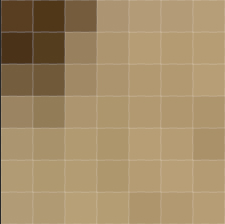
are you able, honestly, to recognize that this is some part of a giraffe’s neck? I don’t think so, right?

Now, If I give you a little more context (and by context, I mean a wider portion of the image):

Figure I.3.4: $50 \times 50$ portion of a girafe's neck

Are you, now, able to Identify that this is probably some portion of a giraffe neck? Maybe you won’t be able to tell that this is some part of the giraffe’s neck but you’ve probably recognized that this picture is “giraffe-related”, right?!

The idea is that, If we only use $7 \times 7$ filters at most, the coefficients that our Neural Network will learn will never be meaningful because it will only rely on a $7 \times 7$ context. If, us, human, we are not able to recognize a giraffe’s neck if we focus only on a $7 \times 7$ portion of the image, how can a Neural Network be able to do it?

Well, the answer is that… The Neural Network cannot do it either! As a human being, to be able to recognize complex structure, the Neural Network needs to pay attention to the context, that is to say to the pixels that are surrounding a central pixel. One way to do it, is to rely on bigger filters. For example, we can imagine a filter of size $51 \times 51$. With such a filter we are sure that we are relying on a broader context. The problem is that the Neural Network will need to learn $51 \times 51 = 2601$ coefficients… And we don’t like this, because the more coefficients need to be learnt, the more complex is the task and the slower the training phase will be. This is why we rely on smaller filter, like $3 \times 3$ filters. But, if that is the case, how the hell can the Neural Network pay attention to a broader context and hence be able to identify complex structures in an image?

Well, the idea is very simple! We use a cascade of small filters! As a picture is better than $1000$ words, here is a picture for you:

Figure I.3.5: cascade of $3 \times 3$ filters

To get the value $X$, we actually used a $3 \times 3$ filter. Hence, $X$ contains information about the $9$ pixels (blue squares). In the same fashion, the red cases in the above image contain information about $9$ pixels each. Finally the value $Y$ is obtained by overlapping a $3 \times 3$ filter over the values that contain information about a broader context.

Hence, here, by using $2$, $3 \times 3$ filters, we were able to focus on a context of size $5 \times 5$ with only $3 \times 3 + 3 \times 3 = 18$ coefficients, while, if we would have used a $5 \times 5$ filter, our neural network would have needed to find… $5 \times 5 = 25$ coefficients!

This is already a good improvement! But the best is when you mix things with $2 \times 2$ max-pooling! Look at this:

Figure I.3.5: $2$ convolutions and one $2 \times 2$ max-pooling

As stated previously, the max-pooling operation doesn’t add any complexity to the model since the Neural Network doesn’t need to learn new coefficients! Yet, by using a max-pooling operation in between 2 convolutions, we were able to focus on a region of size $8 \times 8$ by using only $3 \times 3 + 3 \times 3 = 18$ coefficients (instead of $64$ coefficients!)

This is how, by using small filters in cascade and max-pooling, our Neural Network is able to focus on a broader region while keeping a small number of coefficients to learn!

There is still one part of the Neural Network we haven’t explained yet. This is the Fully Connected component!

the output of the last convolution layer (just before the fully connected layer) is actually a tensor of size $(H’, W’, C’)$ where $H’$, $W’$ and $C’$ are respectively the height, the width and the depth (number of channels) of the tensor. We recall that, here, if $H$, $W$, $C$, are respectively the height, the width and the depth (3 channels) of the input picture we give to the Neural Network then, $H \neq H’$, $W \neq W’$ and $C \neq C’$ since, has we have seen, the $2 \times 2$ max-pooling operation decreases the height and the weight of the input tensor by $2$ and $C’$ the number of filters is actually a hyperparameter, that is to say that, WE choose the value of it. Hence, if our last convolution layer uses $256$ filters then $C’ = 256$

For example if our input picture that we give to our Neural Network is of size $(256, 256, 3)$ ($3$ because our image contains $3$ channels: R, G, B). Then, because we have $3$, $2 \times 2$ max-pooling operations (and because the convolution layers use by default a stride of $1$), the height and the width of our output will be divide $3$ times by $2$, that is to say, $H’ = W’ = 256 / 8 = 32$. For the number of channels, we have said that it depends on the number of filters used in the last convolution layer. If we want it to be $256$, then our output will be of size $(32, 32, 256)$.

Now, recall that the Softmax layer only normalizes the input we give it (The Softmax doesn’t change the size of the tensor). Moreover, we know that our output should be a vector of size $5$ since we want our Neural Network to be able to distinguish between $5$ animals. All in all, it means that the input to the Softmax function should also be a vector of size $5$. But, here we have a 3 dimensional tensor!
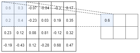
In order to convert this 3D tensor into a vector what we do is that, first, we flatten the tensor. That is to say that we go from a tensor of size $(32, 32, 256)$ to a vector of size $32 \times 32 \times 256 = 262144$. So it’s cool! We have a vector. We don’t need a Fully-Connected layer! Well. Actually, we need a Fully-Connected layer for at least $2$ reasons:

• In our example, the output vector should be of size $5$ because we wanted it to be able to differentiate between $5$ animals. We hence cannot have a vector of size $262144$ as output
• The Neural Network has learned several filters, but it doesn’t yet know how to combine these filters together in order to know what was the animal we just gave him

Here, We want to go from a tensor of size $262144$ to a tensor of size $5$, so the idea is to create a matrix of size $(262144, 5)$ and the Neural Network will have to learn each and every one of the coefficients in this matrix. If you recall your algebra 101 class and matrix multiplication, here is a picture that details what happens:

Figure I.3.6: The Fully-Connected Layer is just a matrix multiplication operation. The coefficients of this matrix are learned by the Neural Network during the training phase

Conclusion

We didn’t enter too much into the mathematical details and I purposely haven’t details everything. This is not the goal of this article and there is a ton of other resources available online that will teach you how a Convolutional Neural Network works. Here, I’ve just wanted to share with you the meaning of each component of a Convolutional Neural Network and why they make sense in order for you to understand how the AlphaGo Zero AI works. Indeed, I feel like, at school, we are taught lot’s of things, but we often skipped the important part: Why ?. Why a convolution operation, why a max-pooling, why this, why that… With this article, I hope I could have helped you have a better understanding of why, and for the newbies, I hope that I could have given you a first intuition and understanding of how a Convolutional Neural Network works. It is really nothing fancy! Believe me, we are far from the SkyNet scenario from the Terminator movie! So, as always, stay tuned for the next article, laymen!